Project
Heston Stochastic Volatility Calibration Engine
Live App: heston-calibration-engine.vercel.app · GitHub: github.com/rcodeborg2311/calibration-engine
Overview
A production-grade Heston stochastic volatility calibration engine that implements the full professional pipeline used by major banks — from FFT-based option pricing to two-phase global-then-local calibration — deployed as a live interactive dashboard. Black-Scholes assumes constant volatility, but real markets exhibit a volatility smile: implied vol varies across strike prices and expiries. The Heston model explains this by letting volatility itself follow a mean-reverting random process correlated with the stock price.
The Heston Model
The model runs two coupled stochastic equations simultaneously:
- Stock price process: the stock moves randomly, but its volatility is controlled by a separate stochastic process v(t)
- Variance process: v(t) mean-reverts toward a long-run average (like a rubber band), with its own random shocks correlated to the stock
Five parameters define the model:
| Symbol | Name | Meaning |
|---|---|---|
| v₀ | Initial variance | How volatile is the stock right now |
| κ (kappa) | Mean-reversion speed | How fast vol snaps back to normal |
| θ (theta) | Long-run variance | What vol settles at over time |
| ξ (xi) | Vol-of-vol | How much volatility itself wobbles |
| ρ (rho) | Correlation | When stock falls, does vol rise? |
FFT Pricing Engine (Carr-Madan)
Option prices are computed via the Carr-Madan (1999) method using FFTW3 — the fastest FFT library in the world:
- Compute the Heston characteristic function φ(u) — a complex-valued mathematical fingerprint of the stock’s future probability distribution
- Apply a 4096-point FFT to convert it into option prices across all strikes simultaneously
- Output: 4096 option prices in a single FFT call
This is the same method used at Goldman Sachs, JPMorgan, and Citadel for real-time options pricing.
Two-Phase Calibration
Given observed market option prices, the engine finds the 5 Heston parameters that minimize the gap between model and market prices (RMSE in basis points, where 1 bps = 0.01% of implied vol).
Phase 1 — Differential Evolution (Global Search): A genetic algorithm that avoids local minima by evolving a population of 15 parameter guesses over 500 generations. Survival-of-the-fittest selection ensures the global optimum region is found before any gradient methods are applied.
Phase 2 — Levenberg-Marquardt (Local Refinement): Switches to a gradient-based optimizer that computes the Jacobian of the residuals and walks downhill precisely to converge on the true minimum.
PDE Solver — Craig-Sneyd ADI
A second independent pricing method for verification: solving the Heston PDE numerically on a 2D grid (stock price × variance) using the Craig-Sneyd Alternating Direction Implicit scheme — the same class of methods used in weather forecasting and fluid dynamics. Time is stepped backwards from expiry to today.
Greeks
All six sensitivities computed via finite differencing:
| Greek | Measures |
|---|---|
| Delta (Δ) | Price change per $1 move in stock — for delta hedging |
| Vega (ν) | Price change per 1% move in vol — for vol trading |
| Theta (Θ) | Price change per 1 day passing — time decay |
| Rho (ρ) | Price change per 1% move in interest rates |
| Vanna | How delta changes as vol changes — second-order hedging |
| Volga | How vega changes as vol changes — vol convexity |
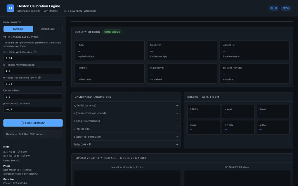
Web Dashboard
An interactive frontend built with Plotly where you can set the true Heston parameters, generate synthetic option prices, run calibration, and inspect the recovered parameters alongside 3D implied volatility surface plots and smile curves.
Architecture
| Layer | Technology |
|---|---|
| Frontend | HTML/CSS/JS + Plotly |
| Hosting | Vercel (static + API proxy) |
| Backend | Python FastAPI on Railway (Docker) |
| Math engine | C++20 binary (subprocess) |
| FFT | FFTW3 |
| Testing | Catch2 (139 unit tests) |
| Benchmarking | nanobench |
Test Coverage
139/139 Catch2 unit tests covering FFT pricing correctness, PDE solver convergence, calibration recovery accuracy, Greek finite-difference consistency, and Feller condition enforcement.